Discrete and Fast Fourier Transforms
Jim Blakey
- Introduction
-
In Digital Signal Processing (DSP) we often would like to break a
complicated sampled waveform down into its most basic component frequencies
in order to analyze or modify it. The set of tools we use for this are called
Fourier Transforms. These are mathematical tools that transform a
waveform in the "Time Domain" (i.e. presented as time .vs. voltage,
time .vs. amplitude, etc) into the "Frequency Domain" (presented as
frequency .vs. that frequency's contribution to the sampled waveform).
This process is often referred to as Frequency or Spectral Analysis.
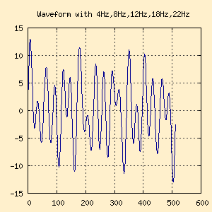
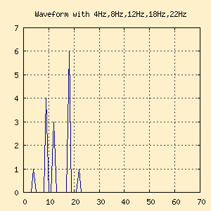
The following figure show the exact same signal, a complex waveform
composed of sine waves at 4Hz, 9Hz, 12Hz, 18Hz and 22Hz. The on the
left the waveform is presented in the Time Domain and on the right in
the Frequency Domain.
 |
 |
| Figure 1-a. Time Domain |
Figure 1-b. Frequency Domain |
The data in the Time Domain is identical to the data in the Frequency
Domain. Converting from the Time Domain to the Frequency Domain is
called Decomposition or a Forward Fourier Transform. Conversion from
the Frequency Domain to the Time Domain is called Synthesis or a
Reverse Fourier Transform. No Information about the signal is lost in
the transforms. The decomposition and synthesis operations are symmetrical.
Most of the discussion you'll find on the internet and in various
books approach Fourier Transforms from a mathematical perspective.
I'm going to try to present this in a more practical engineering
way and try to provide enough information for a basic understanding
of the transforms and hopefully enough code examples to be useful.
As a final note before we dive into the details, there are several
different flavors of Fourier Transforms, depending mainly on how the
input data is represented (among other concerns). For this discussion,
I'll be concentrating on the Discrete Fourier Transform (DFT), of which
the Fast Fourier Transform (FFT) is an example.
The DFT is the most prevalent of the Fourier transforms in DSP because
it takes as its input a discrete, periodic signal. In this case,
discrete means individual discrete samples over time like an Analog-to-Digital
Converter (ADC) provides, and periodic means a repeating waveform, not an
impulse, decaying exponential, or step waveform.
DFT By Correlation
- Basics of Correlation
-
In 1807, Jean Baptiste Joseph Fourier presented a paper to the
Institut de France with the claim that any continuous, periodic
waveform can be represented by the sum of simple sine and cosine waves
of its component frequencies. This was not immediately accepted by
some of his peers however, and led to an almost 15 year disagreement with
the mathematican Joseph Louie Lagrange, who felt that not all
waveforms could be so represented (specifically, waveforms with edges
like square waves). Eventually Fourier's theorm won out and has
become probably the most important tool in DSP.
Since we're discussing the DFT with discrete sampled signals, this
can be expressed more accurately as any given waveform of N samples is
made up of up to N/2 sine and N/2 cosine waves (thank you Mr. Nyquist).
Correlation is the process of finding out how much any given sine wave
relates or contributes to another sine wave. The actual process is fairly
easy. Simply multiply the two waves (point by point), and add the resulting
products.
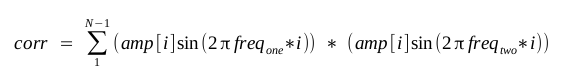
Here's a quick example code snippet that generates two sine waves of
different frequencies and determines their correlation using the above
formula.
	sum_accumulator = 0.0;
	rad_per_sample = ((2 * PI) / sample_size);

	for (i = 0; i < sample_size; i++) {
		sine_one = (amp_one * sinf((rad_per_sample * freq_one * i)));
		sine_two = (amp_two * sinf((rad_per_sample * freq_two * i)));
		sum_accumulator += sine_one * sine_two;
	}

	/*
	** Scale the accumulated value and print
	*/

	sum_accumulator = sum_accumulator / (sample_size / 2);
	printf("The correlation of frequency %d with frequency %d is %f\n",
		freq_one, freq_two, sum_accumulator);
Lets play with this a little to see how it works. If we set the frequencies
of both waves to the same value (freq_one and freq_two
set to 4Hz for example) we would expect a very high degree of correlation
between the two waves. They're identical after all.
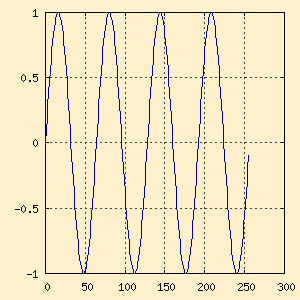 Figure 2-a. 4Hz wave sample
 |
X |
Figure 2-b. 4Hz wave sample |
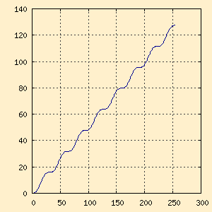
Figure 2-c. Plot of sum_accumulator |
|
When we graph the sum_accumulator value we get an
increasing value that finishes about 128 (the sample size divided by 2).
When we scale this we get a correlation value of 1.003937, for a
high degree of correlation |
As expected, the correlation value (or coefficient) between two identical
4Hz waves is very close to one. Now if we take two dissimilar waves, let's
say a 4Hz and a 9Hz.
|
Figure 3-a. 4Hz wave sample |
X |
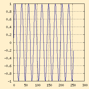 Figure 3-b. 9Hz wave sample
 |
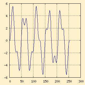 Figure 3-c. Plot of sum_accumulator
 |
|
In the same plot of the sum_accumulator value now
the correlation is 0.00000, as the positive area above 0 on the graph is
canceled out by an equal negative area below 0.
|
The correlation value sum_accumulator is now, for all
practical purposes, zero. A 4Hz and a 9Hz wave do not correlate.
Finally, let's take a more complicated example. Refer back to figure 1-a
above. We had a complex waveform composed of sine waves at 4Hz, 9Hz, 12Hz,
18Hz and 22Hz, all at different amplitudes. If we run our correlation program
to see just how much our 4Hz wave contributes to the overall waveform we get
a correlation value of 0.999805, or very close to one.
This is where the scaling of the sum_accumulator comes
in to play. In the complex waveform, the 4Hz wave contribution had an
amplitude of one. The 9Hz part of the wave had an amplitude of 4, the
12Hz part had an amplitide of 3, etc. By scaling the accumulator value by
the sample size / 2, we get the actual amplitude of that frequency's
contribution to the overall waveform. Scaling the resultant values is
an important part of understanding correlation.
- Phase Contribution
-
In the above discussion the sine waves we were correlating
were all in phase. In our complex example above, we assumed that the 4Hz
wave was in phase with our 4Hz correlation sine wave. What would have
happened if the 4Hz part of the complex wave was a few degrees out of
phase with our test sine wave?
Go back to our simple 4Hz example above. This time let's lag one
of the waves by 30° (or π/6).
|
Figure 4-a. 4Hz wave sample |
X |
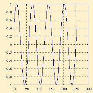 Figure 4-b. 4Hz offset by π/6
 |
The two sine waves still correlate, but to a lesser degree. For the
above with a lag of 30° (π/6) the correlation value was 0.869435,
much less than the 1.0 we had before. If we lag by 45° (π/4) we get
even less correlation at 0.709891. Finally, if we are out of phase by
90° (π/2), the correlation drops to 0.0.
So how do we account for any possible phase? Remember Mr. Fourier's
theorm: any continuous, periodic waveform can be represented by the sum
of simple sine and cosine waves . If we use both a sine and a
cosine wave to correlate, we should be covered for any phase offset. After
all, a cosine wave is just a sine wave 90° out of phase. So as the
correlation of the sine wave drops, the correlation of the cosine part
increases.
So from now on when discussing the Fourier Transforms (either the
DFT or the FFT later), we're going to be working with a sine and a
cosine component for every frequency present in the target waveform.
- A Quick Note About Notation
-
Before I get too far into the actual workings of the DFT, I'm going to
take a brief moment to discuss some basic notational ideas, specifically
related to the sine and cosine components we discussed above. The technical
literature often present the DFT concepts in terms of Complex Numbers, or
numbers containing both a real part and an Imaginary part.
In most cases this is just for mathematical convenience, allowing us to
represent two numbers as one complex value. So let's review.
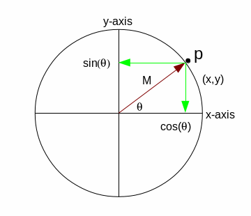
In the above figure, point P can be represented in several different
ways. In the Cartesian system, P is represented by the number pair (x,y).
In Polar Notation, the same point P is represented by an angle and
a magnitude (θ, M). Finally, if we consider the point to be on a unit
circle (radius = 1), then we can reference P as (cos(θ), sin(θ)).
The problem is that each of these requires a numbered pair, x and y,
θ and M, cos(θ) and sin(θ). For convenience,
it would be nice if we could instead deal with P as a single value instead
of a pair. This is where complex numbers come in to play.
A complex number is a number that can not exist in the real world.
Many equations evaluate down to contain the square root of a negative
number (the quadratic equation, for example, often does). The square root
of a negative number can not exist. But why should we let that stop us?
We can represent this non-existant number as a Complex Number, and it
turns out to have some very useful properties.
A complex
number is represented as a real part (containing a Real Number) plus or
minus an imaginary part (containing the square root of a negative number).
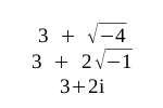
In the complex number above, 3 is the real part. The imaginary part
√-4 is factored out so that it becomes 2 times the square root of -1.
Finally, the √-1 is replaced with the symbol i (or in some
literature, j. We'll use i from here on, as it is more
standard in DSP). Complex numbers are an important part of DSP, electronics,
physics, chaos theory and many other branches of science and engineering.
The great thing about Complex Numbers is that they follow the rules
for addition, subtraction, multiplication and division, and follow many
of the standard mathematical laws. So how can we use them?
Lets again look at the different ways of representing the point P in
the above figure. This time, I'm going to swap out the x-axis for a
Real axis, and the y-axis for an Imaginary axis.
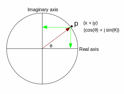
Now we can see that the point P can be represented by the single
complex number x+iy, which can be manipulated with standard
mathematical operations (add, subtract, etc). More importantly from
our DSP perspective, point P can be represented as cos(θ) +
i sin(θ). So now we have a single complex number
that contains both the cosine and sine components of our correlation
exercise above.
Let's take this just one step further. Euler's formula expresses an
important relationship between a cosine and imaginary sine with the natural
exponent e and states that:
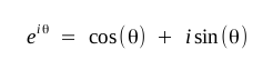
That one single value e i θ
holds both the cosine and sine components of our waveform.
This is the format you'll see in most of the literature on the Fourier
Transforms. But just think of it as a mathematical convenience for
holding cosines and sines.
Since I'm presenting this from a computer engineering perspective,
I'll mostly be using cosines and sines instead of the Euler notation
(until I get to the FFT later). As a nod to the literature, I'm going
to refer to the cosines as the "real" part and the sines as the "imaginary"
part. This is fairly standard.
- Doing The Actual DFT By Correlation
-
Above I discussed how we figure out how much any given frequency
contributes to a sampled waveform. DFT by Correlation is
just the process of repeating that for all possible frequencies. The
Nyquist therom states that for any given sample size of N samples, the
maximum frequency that can be represented is N/2. Therefore, we can
simply just loop from frequency 1 to N/2, testing the cosines and sines
to see how much that frequency contributes. Mathematically, it looks like
this:
In the above analysis equations, x[n] is the time domain
sampled waveform. The freq values will run from 1 to N/2. The arrays
described by real[] and imaginary[] will contain
the cosine and sine components of the wave at that frequency. These
values are known as Fourier Coefficients. In keeping with the standard
notation you'll find in other documents, the cosine component is called
the real part and the sine component is called the imaginary part.
The following code snippet provides an example of this.
	/*
	** Loop through all the possible freqencies in the sample.
	*/

	rad_per_sample = ((2 * PI) / sample_size);
	scale = sample_size / 2;

	for (freq = 0; freq < sample_size/2; freq++) {

		sin_accum = cos_accum = 0.0;
		for (i = 0; i < sample_size; i++) {

			/* cosine contribution.. "real" part */
			cos_val = cosf(rad_per_sample * freq * i);
			cos_prod = cos_val * wave[i];
			cos_accum += (cos_prod / scale);

			/* sine contribution.. "imaginary" part */
			sin_val = sinf(rad_per_sample * freq * i);
			sin_prod = sin_val * wave[i];
			sin_accum -= (sin_prod / scale);

		}
		real_val[freq] = cos_accum;
		imag_val[freq] = sin_accum;
	}
After running this, we are left with N/2 cosine coefficients in the
real_val[] array and N/2 sine coefficients in the imag_val
array. So let's take the complicated waveform from above and run
it through this code snippet.
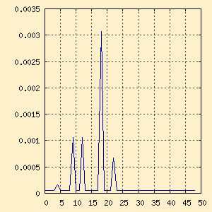
Figure x. Sampled waveform
If we now plot the output values in real_val[] and
imag_val[] we get the following two graphs. Note that I truncated
these graphs at frequency 50 for better presentation.
 |
 |
| Figure x-a. real_val[] (cosine) |
Figure x-b. imag_val[] (sine) |
Now you can kind of see what's going on here between the cosine and
sine components of the input waveform. But the graph becomes much clearer
once we convert the values into Polar Coordinates in the next section.
- Polar Coordinate .vs. Rectangular Coordinates
-
The results of the DFT are an array of cosine and an array of sine
coefficients. When plotted in rectangular coordinates these graphs often
don't make much sense to the human. For a better presentation, these
values are often converted to Polar Coordinates before graphing.
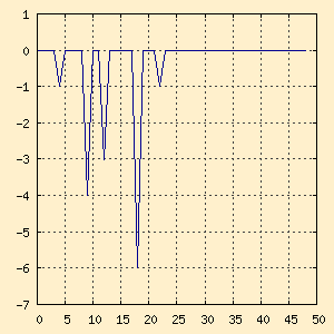
 |
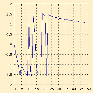 |
| Figure x-a. Magnitude (polar) |
Figure x-b. Phase (polar) |
These are the same graphs as figures x and x, just presented in
polar form. Notice in the Magnitude graph how easy it is to pick out
the component frequencies and their exact contributions to the original
sampled waveform. The Phase graph shows any phase differences, and
is harder to understand.
Usually, programs that do DFTs will keep the values internally in
rectangular form as the math is easier, and convert to polar only for
display.
Let's go back and review figure x above where the unit circle is
presented. In that figure, point P can be represented by the cosine
and sine values of theta. That same point can also be presented by a vector
consisting of a magnitude (length) and phase (angle theta). The general
conversion between the coordinate systems is:
 |
and |
 |
In our case, the translation of the real (cosine) and imaginary
(sine) to polar looks like
 |
and |
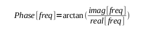 |
And to translate back to rectangular coordinates:
 |
and |
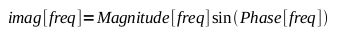 |
Although in principle the conversion between coordinate systems is easy,
there are several important things to watch out for. I've provided another
code snippet that does the conversion. The important issues with the
conversions are documented in the code.
/* ----------------------------------------------------------------
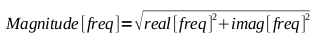
** polarMagnitude()
**
** returns polar coordinate magnitude for given real/imag
**
** ----------------------------------------------------------------
*/
float
polarMagnitude(float r, float i)
{
float mag;
mag = sqrtf(powf(r,2) + powf(i,2));
return mag;
}
/* ----------------------------------------------------------------
** polarPhase()
**
** returns polar coordinate phase for given real/imag
**
** ----------------------------------------------------------------
*/
float polarPhase(float r, float i)
{
float phase;
/*
** if the real part == 0.0, that just means that the phase is exactly 90
** or -90. Not a problem, just handle:
*/
if (r == 0.0) {
if (i > 0.0) {
phase = PI/2;
} else {
phase = -PI/2;
}
} else {
phase = atanf(i / r);
}
/*
** settle sign ambiguity on phase. If real and imaginary are both
** negative the returned arctan needs 180 subtracted. If the real
** is negative and imaginary is positive, add 180.
*/
if ((r < 0) && (i < 0)) {
phase = phase - PI;
}
if ((r < 0.0) && (i > 0.0)) {
phase = phase + PI;
}
return phase;
}
- Synthesis: Recreating The Time Domain From The Frequency Domain
-
Synthesis is the process of converting samples from the frequency domain
back into the time domain (reverse-DFT is another way to look at it). This
is done in the same way correlation is done, by running through the real and
imaginary parts rebuilding the cosine and sine waves for each frequency. The
formula for this is
Fast Fourier Transforms
- Basics
The problems with the DFT by correlation described above should be
fairly obvious: it is slow and doesn't scale well with larger sample sizes.
It basically has an efficency of O(2N2), meaning that for
a sample size of 256 bytes, over 131,000 calculations must be performed
The larger the sample size, the number of calculations increases
exponentially. For a sample size of 1024 (only 4 times larger that the
256 samples) well over two million calculations need to be performed.
In 1965, J. W. Cooley and John Tukey published a paper describing what
is now the most common form of the Fast Fourier Transform (although several
others, including Gauss, had come up with varients of it before). This
algorithm increases the efficiency by orders of magnitude and scales
much better. The FFT has an efficency of O(N log2 N), meaning
that the 256 byte sample takes only about 2000 calculations, and the 1024
takes just over ten thousand. This is a huge increase in efficiency.
The math behind the FFT is fairly complicated and I'm only going to touch
on it enought to give a general understanding of how it works and what the
example code is doing. If you want to delve deeper into it, there are many
great books and resources on the Internet. For this part of the discussion
I'll be using the Euler notation described above, as it makes it easier to
understand what's happening. It's also the format most commonly used
in the technical documentation. Just keep in mind that the e notation
is really just describing cosines and sines like we did in correlation.
You can use Euler's Identity to rewrite the equations in terms of cosines
and sines if you're more comfortable with the triginometric flavors.
The FFT algorithm is a version of the DFT that exploits the properties
of Symmetry and Periodicity of waveforms to reduce what are effectively
redundant calculations.
| Symmetry | 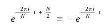 |
| Periodicity | 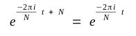 |
These properties allow us to use a "divide and conquer" approach
to the FFT. We can take an N-point DFT and divide it into 2 N/2-point
DFTs. These can then be further divided over and over until there are
N 1-point DFTs. This process is called Radix-2 Decimation In Time
and is the basis of the FFT. The math looks like this:
Starting with the DFT Basis function for a sample size N, where N is
an even power of 2:
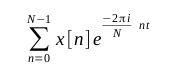
We can rewrite this using what is sometimes called the Danielson-Lanczos
lemma as the sum of two shorter DFTs, each of length N/2. The left side is
created using the even numbered points from the original sample and the right
side is created using the odd numbered points. The right side is multiplied
by a complex root-of-unity factor, called a "twiddle factor".
Now this process is repeated, breaking the left hand side of the equation
(what were the even numbered points of the original sample) further down into
its even/odd pairs, then the right hand side of the equation (the original odd
numbered sample points) into its even/odd pairs. This is repeated until we
have N individual DFTs of just one sample each.
Computationally, the FFT Decimation In Time is performed in two stages.
First the sample is recursively broken into smaller and smaller even/odd
samples until it becomes N samples of size one. This is a form of
Interleaved Decomposition. Then the samples are recombined in the
reverse order, with the additional multiplication by the complex twiddle
factor in a pattern known as the FFT Butterfly.
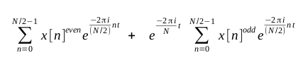
- Step 1: Decomposing the Time Domain Signal
-
Decomposing a signal of N points in the time domain involves turning it
into N signals of one point. This is called interlaced decomposition.
The method is to take the signal and convert it into two signals, one of the
even members of the parent signal and one of the odd members. Then take those
two results and perform the same operation. Repeat. The following diagram
shows this
This is obviously a process that lends itself to recursion, and there
are many FFT implementations that use recursion to accomplish this. However,
it turns out that there is a simpler way to do this if the sample size
is an even power of 2. Since this step is actually nothing more than a
simple re-ordering of samples it can be done "in place" by using a
Bit Reversal Sort algorithm.
The Bit Reversal Sort takes advantage of an interesting property of
the indicies of the sample array. If you just reverse the order of the
bits in the index (in binary) you have the index of the value you want
to swap with. For example, index 5 (0101) swaps with index 10 (1010),
index 3 (0011) swaps with index 12 (1100), etc.. The table below shows
this:
| Index | Binary | New Index | Binary |
| 0 | 0000 | 0 | 0000 |
| 1 | 0001 | 8 | 1000 |
| 2 | 0010 | 4 | 0100 |
| 3 | 0011 | 12 | 1100 |
| 4 | 0100 | 2 | 0010 |
| 5 | 0101 | 10 | 1010 |
| 6 | 0110 | 6 | 0110 |
| 7 | 0111 | 14 | 1110 |
Etc...
If your sample size is not an even power of two, just pad it out
with zeros to the next power of 2 size. This will not cause any
problems, as it will just be considered a zero frequency component
of the waveform.
The following code snippet does this bit reversal.
/* -------------------------------------------------------------------
** bitReversalSort()
**
** Does the bit reversal sort of the supplied input array. This
** is a re-write in C of the BASIC algorithm supplied from
** www.dspguide.com in Chapter 12.
** Note that the arrays are sorted in place.
**
** -------------------------------------------------------------------
*/
int
bitReversalSort(int count, float real_val[], float imag_val[])
{
int index, newindex, k;
float tempR, tempI;

        newindex = count / 2;
        for (index = 1; index < count - 2; index++) {
/*
** only swap if we haven not swapped this one already
*/
                if (index < newindex) {
                        tempR = real_val[newindex];
                        tempI = imag_val[newindex];

                        real_val[newindex] = real_val[index];
                        imag_val[newindex] = imag_val[index];

                        real_val[index] = tempR;
                        imag_val[index] = tempI;
                }
/*
** calculate the next newindex
*/
                k = count / 2;
                while ( k <= newindex) {
                        newindex = newindex - k;
                        k = k / 2;
                }
                newindex = newindex + k;
        }
        return 0;
}
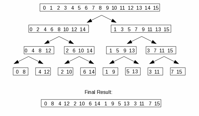
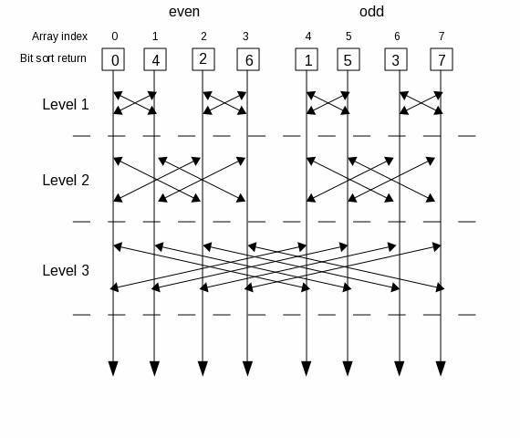
- Step 2: Re-composing the signal in the Frequency Domain
-
After the Bit Reverse Sort algorithm, we're left with N signals
each of sample size 1. These are effectively in the frequency domain
now, as the frequency of a single sample signal is itself.
Now we have to reverse the interlaced decomposition we did in the time
domain above by interlacing the values again in the frequency domain. Each
time we combine two components, we multiply by the "twiddle factor" described
above. The pattern of re-combining is called the FFT Butterfly:
Note the multiplication of one of the terms with the complex sinusoid
twiddle factor and the inversion of the sign. The complex sinusoid is
calculated differently at each level, depending on how many elements are
in that level.
Now the difficult part is doing the actual interlacing work. We can
not use the bit reversal trick with indicies that we used in the
decomposition so we have to loop through the hard way, recombining pairs
using the FFT Butterfly. The process looks like this:
Note: The above diagram leaves out the twiddle factor multiplication at
each level for simplicity, as it was described in the butterfly diagram.
The following code snippet is an example of the FFT butterfly
/* ------------------------------------------------------------------
** FFTButterfly()
**
** This routine does a Discrete Fourier Transform using the Fast
** Fourier Transfor (FFT) algorithm described by Cooley and Tukey.
** This expects both the real and imaginary input waveforms to have
** already been run through the interlaced decomposition bit reversal
** algorithm. This will recompose in the frequency domain using the
** FFT butterfly.
**
** ------------------------------------------------------------------
*/

void FFTButterfly(int count, float real_val[], float imag_val[])
{

int numLevels;
int samplesInLevel;
int level;
float butterflyR, butterflyI;
float sinusoidR, sinusoidI;
float tR, tI, tempR;
int i, j, IP;

/*
** For each 'level' of decomposition done by the bit reversal sort
** (and there are log2(count) of them) loop do ...
*/

        numLevels = (int) (logf(count) / logf(2));
        for (level = 1; level <= numLevels; level++) {

                samplesInLevel = (int) powf(2,level);
/*
** calculate the complex sinusoid twiddle factor that we are using in
** the butterfly calculation for this level.
*/
                butterflyR = 1;
                butterflyI = 0;
                sinusoidR = cosf(PI / (samplesInLevel / 2));
                sinusoidI = - sinf(PI / (samplesInLevel / 2));

                for (j = 1; j <= (samplesInLevel / 2); j++) {
/*
** This loop does the actual FFT butterfly operation for each pair of points
*/
                        for (i = (j - 1); i <= (count - 1); i = i + samplesInLevel) {

                                IP = i + (samplesInLevel / 2);
                                tR = real_val[IP] * butterflyR - imag_val[IP] * butterflyI;
                                tI = real_val[IP] * butterflyI + imag_val[IP] * butterflyR;

                                real_val[IP] = real_val[i] - tR;
                                imag_val[IP] = imag_val[i] - tI;

                                real_val[i] = real_val[i] + tR;
                                imag_val[i] = imag_val[i] + tI;
                        }
/*
** recalculate the new butterfly value
*/
                        tempR = butterflyR;
                        butterflyR = tempR * sinusoidR - butterflyI * sinusoidI;
                        butterflyI = tempR * sinusoidI + butterflyI * sinusoidR;
                }
        }
        return;
}
- Putting It All Together: Code Sample For Complete FFT
-
The following is a small test routine to demonstrate the Bit Reversal
Sort and FFT Butterfly routines. The calling program would read in a
waveform from some source (file, socket, DSP chip, etc) and perform
the necessary floating point scaling. This routine shows how to
change the input real floating point waveform set into the Real and
Imaginary arrays for the FFT.
The results are kept in the Real and Imaginary arrays and are just
printed out in the Polar magnitude format for easier understanding
/* ------------------------------------------------------------------
** test_FFT()
**
** test driver for FFT. Input is sample size and waveform, waveform
** changed inplace
**
** ------------------------------------------------------------------
*/
void
test_FFT(int sample_size, float wave[])
{
float imag_val[D_MAX_SAMPLES];
float real_val[D_MAX_SAMPLES];
int i;

/*
** convert the input waveform, set the imaginary part to zeros
*/
        for (i = 0; i < sample_size; i++) {
                real_val[i] = wave[i];
                imag_val[i] = 0.0;
        }

/*
** call the bitReversalSort() routine to do the interlaced decomposition
** of the waveform. Then call the FFT butterfly to re-compose in the
** frequency domain
*/
        bitReversalSort(sample_size, real_val, imag_val);

        FFTButterfly(sample_size, real_val, imag_val);
/*
** Print results in index, real, imaginary, polar magnitude and phase
** Note: Only print sample_size / 2 results. These are the valid ones.
** The FFT is symetrical around the sample_size/2 point, so anything
** above that is repeated data.
*/
        for (i = 0; i < sample_size/2 ; i++) {
                printf("%2d  %.4f  %.4f  %.4f  %.4f\n", i,  real_val[i], imag_val[i],
                        polarMagnitude(real_val[i], imag_val[i]),
                        polarPhase(real_val[i], imag_val[i]) );
        }
        printf("\n");

        return;
}
|
